
Static Timing Analysis (STA) is the method used to verify that every timing path in a digital design meets its timing requirements, without running a single simulation vector. In modern STA in VLSI flows, it is run at every stage – after synthesis, after placement, after Clock Tree Synthesis (CTS) and after routing – and a design cannot be signed off for tape-out until STA is clean across all required corners and modes.
In this tutorial we cover what static timing analysis is, how timing paths are formed, how setup and hold checks work, how slack is calculated, the difference between OCV, AOCV and POCV, how CRPR (also called CPPR) removes pessimism with a worked numeric example, timing corners, and the most common STA interview questions.
What is Static Timing Analysis?
Static timing analysis is a technique that computes the worst-case (and best-case) arrival time of signals at every timing endpoint of a circuit by adding up cell delays and net delays along each path, and then compares them with the required time derived from the clock. It is called static because it does not depend on input stimulus: instead of simulating functional vectors, the tool analyses the structure of the netlist and checks all paths exhaustively.
An STA tool (for example Synopsys PrimeTime, Cadence Tempus, or the timing engines inside implementation tools) needs these inputs:
- Gate-level netlist – the design to be analysed.
- Liberty (.lib) timing libraries – cell delays, transitions, setup/hold and other constraint tables for each PVT corner.
- SDC constraints – clocks, generated clocks, input/output delays, false paths, multicycle paths, clock uncertainty, etc.
- Parasitics (SPEF) – extracted RC of the nets after routing (before routing, the tool estimates wire load).
- Derates / variation data – OCV derates, AOCV tables or POCV/LVF data.
For background on the inputs used during implementation, see Synthesis Overview and Inputs and Physical Synthesis.
STA vs Dynamic Timing Analysis
| Aspect | Static Timing Analysis | Dynamic (Simulation-based) Timing |
|---|---|---|
| Input vectors | Not required | Required |
| Coverage | All structural paths | Only paths exercised by the vectors |
| Speed | Fast, scales to large SoCs | Slow on large designs |
| Functional check | No – checks timing only | Yes – checks function and timing |
| False paths | Must be declared through constraints | Naturally ignored if never sensitised |
Timing Paths in STA
Every timing path has a start point and an end point. Start points are clock pins of sequential cells or primary input ports; end points are data input pins of sequential cells or primary output ports. This gives four basic path types:
- Input to register (in2reg) – from an input port to a flip-flop D pin.
- Register to register (reg2reg) – from a flip-flop clock pin to another flip-flop D pin. This is the most common path type.
- Register to output (reg2out) – from a flip-flop clock pin to an output port.
- Input to output (in2out) – a purely combinational feed-through path.
Besides these data paths, STA also analyses clock paths (from the clock source to clock pins), clock-gating paths (to the enable pin of a gating cell – see Integrated Clock Gating (ICG) Cell) and asynchronous paths (to reset/set pins, checked with recovery and removal time).
A reg2reg path has three parts: the launch clock path (clock source to launch flop), the data path (launch flop CK→Q plus combinational logic up to the capture flop D pin) and the capture clock path (clock source to capture flop).
Arrival Time, Required Time and Slack
- Arrival Time (AT) – when the data actually reaches the endpoint: launch clock latency + clock-to-Q delay + combinational and net delays.
- Required Time (RT) – when the data must arrive for correct capture, derived from the capture clock edge, capture clock latency, the library setup/hold value and uncertainty.
- Slack – the margin between them. Positive slack means the path meets timing; negative slack means a violation.
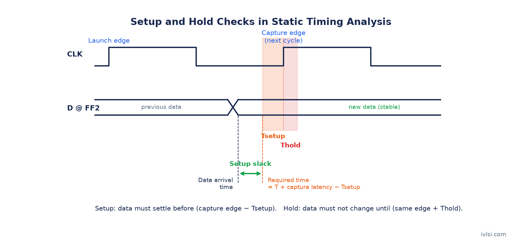
Setup slack = Required time - Arrival time
Hold slack  = Arrival time - Required time
Two summary metrics appear in every timing report: WNS (Worst Negative Slack), the slack of the single worst path, and TNS (Total Negative Slack), the sum of negative slack over all violating endpoints. WNS tells you how far you are from the target frequency; TNS tells you how widespread the problem is.
Setup and Hold Checks
Setup Check
Setup time is the minimum time the data must be stable before the active clock edge at the capture flop. The setup check makes sure data launched on one clock edge reaches the capture flop before the next capture edge (minus the setup time). It is a max-delay check, so the tool uses the slowest (late) data path.
Setup:  Tlaunch + Tck2q + Tcomb(max)  <=  Tperiod + Tcapture - Tsetup - Tuncertainty

Setup slack = (Tperiod + Tcapture - Tsetup - Tunc) - (Tlaunch + Tck2q + Tcomb)
Hold Check
Hold time is the minimum time the data must remain stable after the active clock edge. The hold check makes sure data launched on a clock edge does not race through and corrupt the data being captured on the same edge at the capture flop. It is a min-delay check, so the tool uses the fastest (early) data path.
Hold:  Tlaunch + Tck2q + Tcomb(min)  >=  Tcapture + Thold + Tuncertainty

Hold slack = (Tlaunch + Tck2q + Tcomb) - (Tcapture + Thold + Tunc)
Note that the hold check does not include the clock period. That is why hold violations cannot be fixed by slowing the clock, while setup violations can – an important point that comes up in interviews.
Effect of Clock Skew
Skew = capture clock latency − launch clock latency. Positive skew (capture clock arrives later) helps setup but hurts hold; negative skew helps hold but hurts setup. Deliberately using skew to borrow margin is called useful skew.
Common Ways to Fix Violations
| Setup violation fixes | Hold violation fixes |
|---|---|
| Upsize drivers / use lower-Vt cells | Insert delay buffers or delay cells on the data path |
| Restructure or reduce logic depth | Downsize cells / use higher-Vt cells on the data path |
| Buffer long nets, fix bad transitions | Adjust clock skew (reduce capture latency where safe) |
| Useful skew, better placement | Detour routing in rare cases |
| Pipelining or relaxing the frequency target | Correct missing multicycle/false path constraints |
Placement and routing quality directly affect these numbers; see Performance (Timing) and Placement Optimization. Crosstalk can also add or remove delay on a net – covered in Signal Integrity and Crosstalk.
On-Chip Variation: OCV vs AOCV vs POCV
Even on a single die, two identical cells do not have exactly the same delay because of local process, voltage and temperature variation. On-Chip Variation (OCV) modelling makes STA pessimistic in the right direction: for a setup check, the launch clock and data paths are made slower (late) and the capture clock path faster (early); for a hold check it is the opposite.
OCV (flat derate)
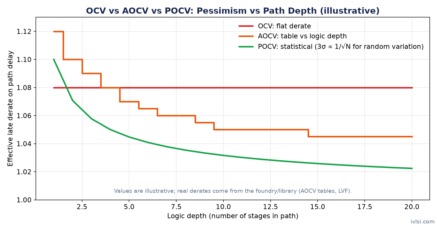
Classic OCV applies a single derate factor to all cells or nets, for example a late derate of 1.05 and an early derate of 0.95. It is simple but very pessimistic for long paths, because random variations along many stages partly cancel out in reality, while a flat derate assumes every stage is worst-case.
AOCV (Advanced OCV)
AOCV uses derate tables indexed by logic depth (number of cell stages) and often by distance (the bounding box of the path). Deeper paths get a smaller derate because random variation averages out over more stages. This removes much of the excess pessimism of flat OCV.
POCV (Parametric OCV) / SOCV
POCV models each cell delay as a statistical distribution with a mean (μ) and standard deviation (σ). Sigmas are combined statistically along the path (root-sum-square for independent random variation), and the final path delay is taken at a chosen sigma level, typically 3σ. The variation data comes from Liberty Variation Format (LVF) or a single σ coefficient per cell. Synopsys tools commonly call it POCV and Cadence tools SOCV.
| Parameter | OCV | AOCV | POCV / SOCV |
|---|---|---|---|
| Variation model | Single flat derate | Derate table vs depth (and distance) | Statistical μ and σ per cell/arc |
| Path depth awareness | No | Yes | Yes (inherently, via statistics) |
| How variation accumulates | Linearly (worst case every stage) | Linearly, reduced derate for deeper paths | Statistically (RSS of σ) |
| Pessimism | Highest | Medium | Lowest (most realistic) |
| Library data needed | Derate values | AOCV tables | LVF or σ coefficients |
| Typical usage | Older nodes, early estimates | Mid nodes (e.g. 40–20 nm) | Advanced nodes, sign-off |
| Runtime | Lowest | Low | Slightly higher |
CRPR / CPPR: Clock Reconvergence Pessimism Removal
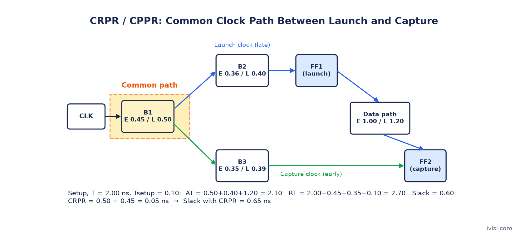
When OCV derates are applied, the launch clock path is calculated late and the capture clock path early for a setup check. But launch and capture clock paths usually share a common segment from the clock source up to a common point (the last cell shared by both paths). A physical cell cannot be both slow and fast at the same instant, so applying different derates to the shared segment adds artificial pessimism.
CRPR (Synopsys term) or CPPR – Common Path Pessimism Removal (Cadence term) gives this pessimism back as a credit:
CRPR credit = Late arrival at common point - Early arrival at common pointFor a setup check the credit is added to the slack. For a hold check (same-edge launch and capture) the same idea applies. When launch and capture happen on different edges, tools may only remove the static part of the variation and not the dynamic (e.g. crosstalk) part, as the common path is not switching at the same instant.
Worked CRPR Example
Consider a reg2reg path from FF1 to FF2 with a clock period of 2.00 ns. The clock passes through a common buffer B1, then splits: B2 drives FF1 (launch), B3 drives FF2 (capture). Delays with OCV derates already applied:
| Element | Early delay (ns) | Late delay (ns) |
|---|---|---|
| B1 (common path) | 0.45 | 0.50 |
| B2 (launch branch) | 0.36 | 0.40 |
| B3 (capture branch) | 0.35 | 0.39 |
| FF1 CK→Q + logic (data path) | 1.00 | 1.20 |
| FF2 setup time | – | 0.10 |
Step 1 – Arrival time (late, for setup): 0.50 (B1) + 0.40 (B2) + 1.20 (data) = 2.10 ns
Step 2 – Required time (early capture clock): 2.00 (period) + 0.45 (B1) + 0.35 (B3) − 0.10 (setup) = 2.70 ns
Step 3 – Slack without CRPR: 2.70 − 2.10 = 0.60 ns
Step 4 – CRPR credit: B1 late − B1 early = 0.50 − 0.45 = 0.05 ns
Step 5 – Slack with CRPR: 0.60 + 0.05 = 0.65 ns
The 0.05 ns was pure pessimism caused by treating B1 as both slow and fast. On a real design with long shared clock trunks, CRPR can recover a meaningful amount of slack, which is why it is always enabled in sign-off (for example set timing_remove_clock_reconvergence_pessimism true in PrimeTime).
Timing Corners and Modes
Cell and wire delays change with Process, Voltage and Temperature (PVT). STA is run at multiple corners so that the chip works across the whole operating range:
| Corner | Process / Voltage / Temperature | Mainly used for |
|---|---|---|
| SS (slow-slow) | Slow devices, low voltage, low or high temperature | Setup (max delay) |
| FF (fast-fast) | Fast devices, high voltage, low or high temperature | Hold (min delay) |
| TT (typical) | Typical devices, nominal voltage, room temperature | Power and reference analysis |
| SF / FS | Skewed NMOS/PMOS | Special checks (e.g. memories, level shifters) |
At advanced nodes, temperature inversion means that at low voltage a cell can be slower at low temperature than at high temperature, so both cold and hot slow corners are analysed. Interconnect also has its own RC corners such as Cworst, Cbest, RCworst and RCbest. Combining PVT corners, RC corners and functional/test modes gives the MCMM (Multi-Corner Multi-Mode) scenario set used in implementation and sign-off.
Other Checks Done in STA
- Max transition, max capacitance and max fanout (design rule checks)
- Minimum pulse width and clock duty cycle – see Duty Cycle & Pulse Width
- Recovery and removal checks on asynchronous pins
- Clock gating setup/hold checks
- Latch time borrowing
- Signal integrity (crosstalk delta delay and noise)
Most STA work involves parsing reports and writing small scripts. Our TCL tutorial series and Practical Exposure to writing TCL are a good companion for this.
Static Timing Analysis Interview Questions
Q1. Why is it called static timing analysis?
Because it checks timing without input vectors, by analysing all structural paths of the netlist.
Q2. Can a hold violation be fixed by reducing the clock frequency?
No. The hold check is between launch and capture on the same edge and does not depend on the clock period. Setup violations can be fixed by reducing frequency.
Q3. Which corner is critical for setup and which for hold?
Usually the slow corner (SS, low voltage) for setup and the fast corner (FF, high voltage) for hold, though temperature inversion means several temperatures must be checked.
Q4. How does positive skew affect setup and hold?
Positive skew (capture clock later) improves setup slack and degrades hold slack.
Q5. What is the difference between WNS and TNS?
WNS is the worst slack of any single path; TNS is the sum of all negative slacks.
Q6. What is a false path and a multicycle path?
A false path is a structural path that is never functionally exercised, so it is excluded from timing. A multicycle path is allowed more than one clock cycle to propagate; the hold check usually has to be adjusted along with the setup multiplier.
Q7. Why do we need CRPR?
Because OCV derates treat the common clock path as both early and late, which is physically impossible. CRPR removes this pessimism.
Q8. What is the difference between OCV and POCV?
OCV applies a flat derate; POCV models delay statistically with μ and σ and combines variation along the path, giving less pessimistic results.
Q9. What happens if both setup and hold fail on the same path?
Fixing one usually worsens the other. Check the constraints and clock skew first; often the real issue is a large skew or wrong constraint rather than the data path.
FAQ
What is STA in VLSI?
STA in VLSI is the process of verifying that all timing paths of a chip meet setup, hold and other timing requirements across corners and modes, without simulation.
Which tools are used for static timing analysis?
Common sign-off tools include Synopsys PrimeTime and Cadence Tempus; implementation tools such as Innovus and ICC2 also contain timing engines, and OpenSTA is an open-source option.
Is STA done before or after routing?
Both. It is run after synthesis, placement and CTS with estimated parasitics, and final sign-off STA is run after routing with extracted SPEF.
What is the difference between CRPR and CPPR?
They are the same concept. CRPR is the term used by Synopsys and CPPR by Cadence.
Related iVLSI tutorials: Setup and Hold Violations: Examples and Fixes | Antenna Effect in VLSI
Conclusion
Static timing analysis is the backbone of timing sign-off. Once you understand timing paths, the setup and hold equations, slack, variation models like OCV, AOCV and POCV, CRPR and timing corners, you can read any timing report with confidence and debug violations systematically. Continue with Clock Tree Synthesis (CTS) and Recovery and Removal Time to strengthen your timing fundamentals.